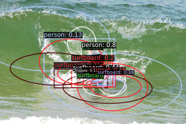
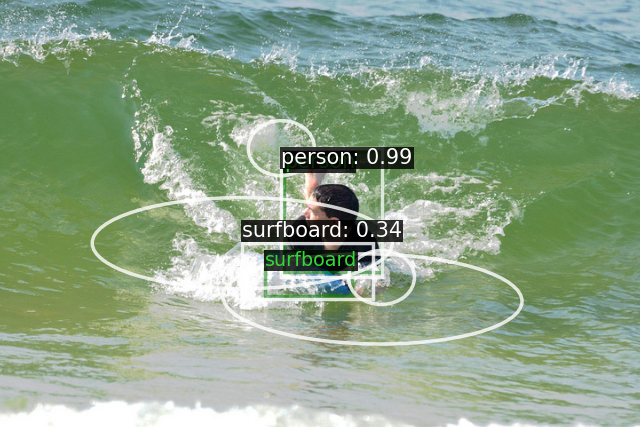
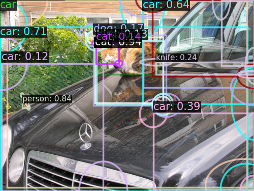
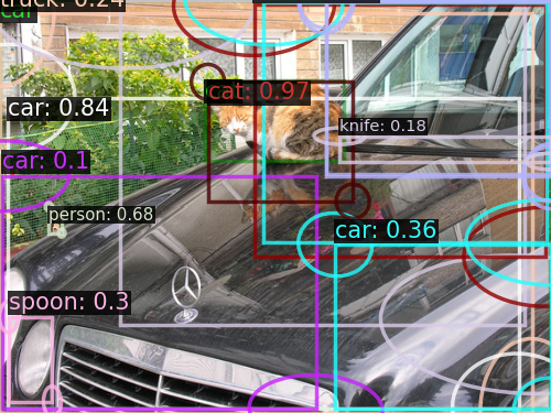
Object Detection as Probabilistic Set Prediction

Training and evaluation of probabilistic object detectors

Core idea

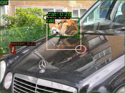
We take the perspective that object detection is a set prediction task, and generalize it to probabilistic object detection. Given an image \(\mathbf{X}\) the model predicts a distribution over the set of objects \(\mathbb{Y}\), i.e., \(f_{\theta} (\mathbb{Y} | \mathbf{X})\).

We use the Random Finite Set (RFS) formalism to model the set of objects. Evaluation of \(f_{\theta} (\mathbb{Y} | \mathbf{X})\) is fully differentiable, and can be used to both for training and evaluation of probabilistic object detectors. Specifically, we use the negative log-likelihood (NLL) as a proper scoring rule for evaluating and training the models.

Left: results by training with existing approaches . Right: results when training with the proposed method. Our loss function encourages more plausible predictions, with fewer false positives, and better described uncertainty.

Abstract

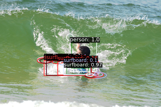
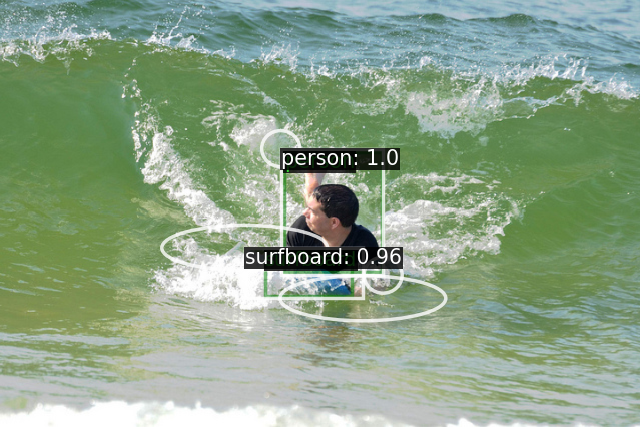
Accurate uncertainty estimates are essential for deploying deep object detectors in safety-critical systems. The development and evaluation of probabilistic object detectors have been hindered by shortcomings in existing performance measures, which tend to involve arbitrary thresholds or limit the detector’s choice of distributions. In this work, we propose to view object detection as a set prediction task where detectors predict the distribution over the set of objects. Using the negative log-likelihood for random finite sets, we present a proper scoring rule for evaluating and training probabilistic object detectors. The proposed method can be applied to existing probabilistic detectors, is free from thresholds, and enables fair comparison between architectures. Three different types of detectors are evaluated on the COCO dataset. Our results indicate that the training of existing detectors is optimized toward non-probabilistic metrics. We hope to encourage the development of new object detectors that can accurately estimate their own uncertainty.

Background

When we solve classification tasks, we typically train a model using the cross-entropy loss. By doing so, we implicitly assume the true label to be a random variable with a categorical distribution.

A model is trained to predict the probability of each class given an image.

When we solve a regression task, we might use the L2-loss. By doing so, we implicitly assume the true label to be a random variable with a Gaussian distribution.

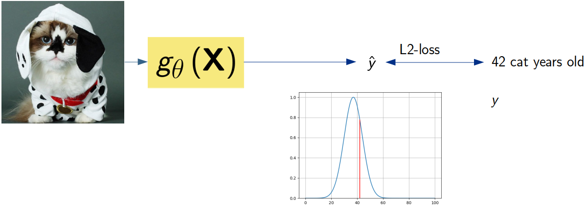
A model is trained to predict the age of a cat, given an image.

In both cases, we assume that the true label is a single random variable with a known distribution, and we train the model to predict the parameters of that distribution. We argue that we should do the same for object detection.

Object detection as a set prediction task

In this work, we view the set of objects in a an image as a single random variable \(\mathbb{Y}\).

The task of the model is to predict the distribution over the set of objects \(f_{\theta} (\mathbb{Y} | \mathbf{X})\), where \(\mathbf{X}\) is the image.

The evaluation can be done using standard tools like negative log-likelihood (NLL)

\[\mathcal{L}_{\text{NLL}} (\mathbb{Y}, f_{\theta} (\mathbb{Y} | \mathbf{X})) = - \log f_{\theta} (\mathbb{Y} | \mathbf{X})\]

The training can be done using the same loss function.

Modeling a single object

To model a single object, we need to capture the characteristics of the object. We do so by modelling each object as a Bernoulli Random Finite Set \(f_{B}(\mathbb{Y})\).

Existance. First off, we need to capture if the object is present or not.

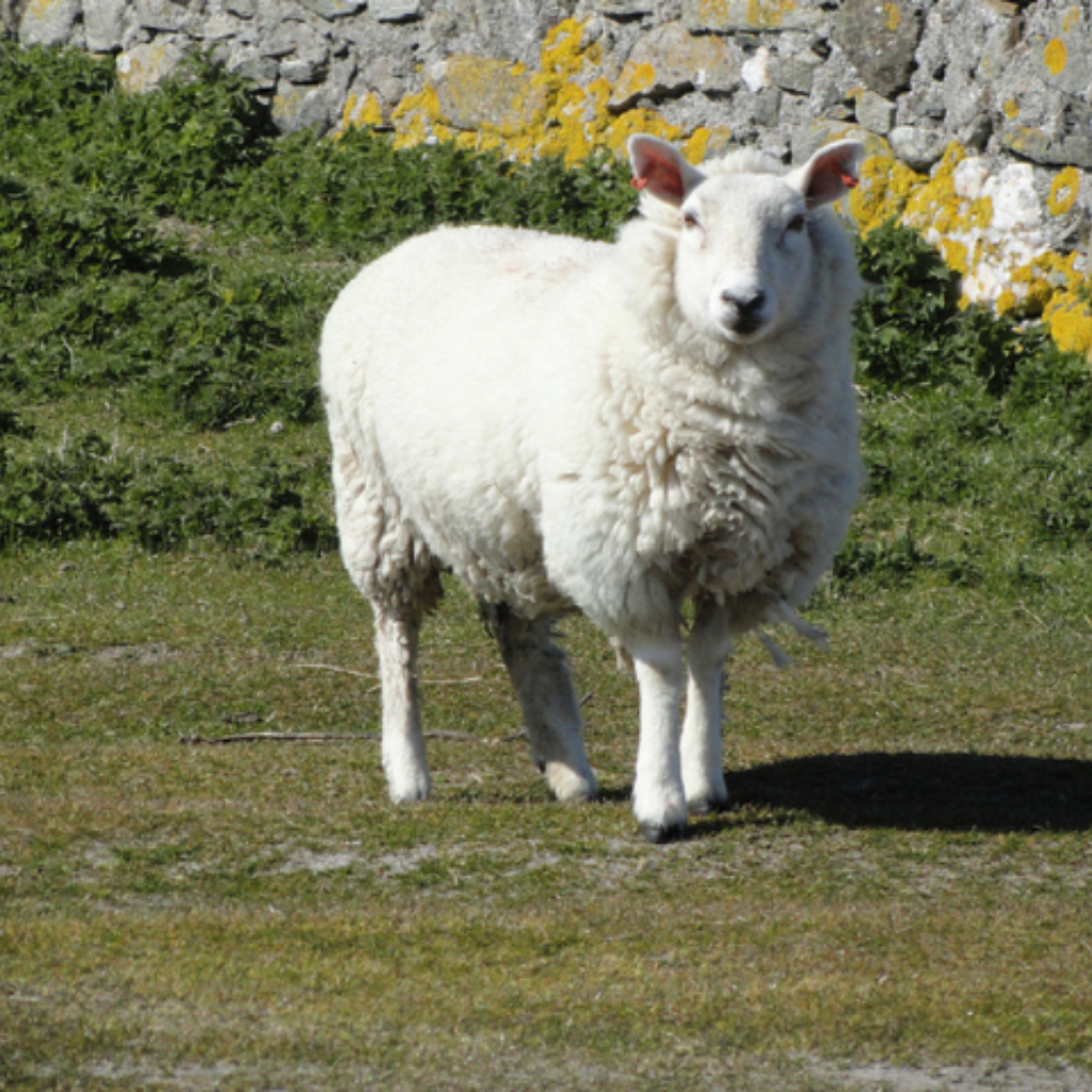
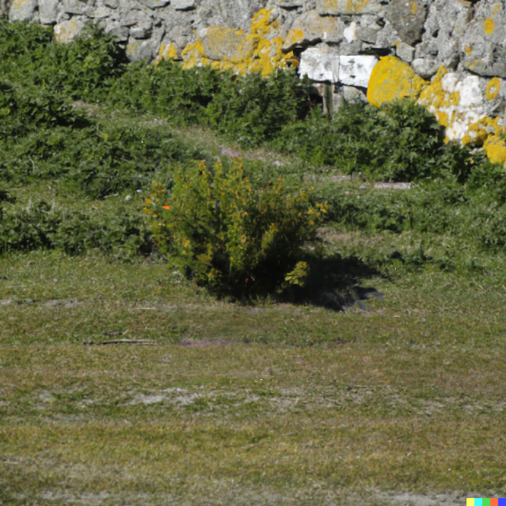
This is captured in the density function \(f_{B}(\mathbb{Y})\) as:

\[f_B(\mathbb{Y}) = \begin{cases} 1 - r & \text{if } \mathbb{Y} = \emptyset, \\ r & \text{if } \mathbb{Y} = \{ \mathbf{y} \}, \\ 0 & \text{if } |\mathbb{Y}| > 1 \end{cases}\]

where \(y\) is the object and \(r \in [0,1]\) an existance probability, i.e., probability of the set containing an element.

Size and class. Next, objects can have different sizes and classes

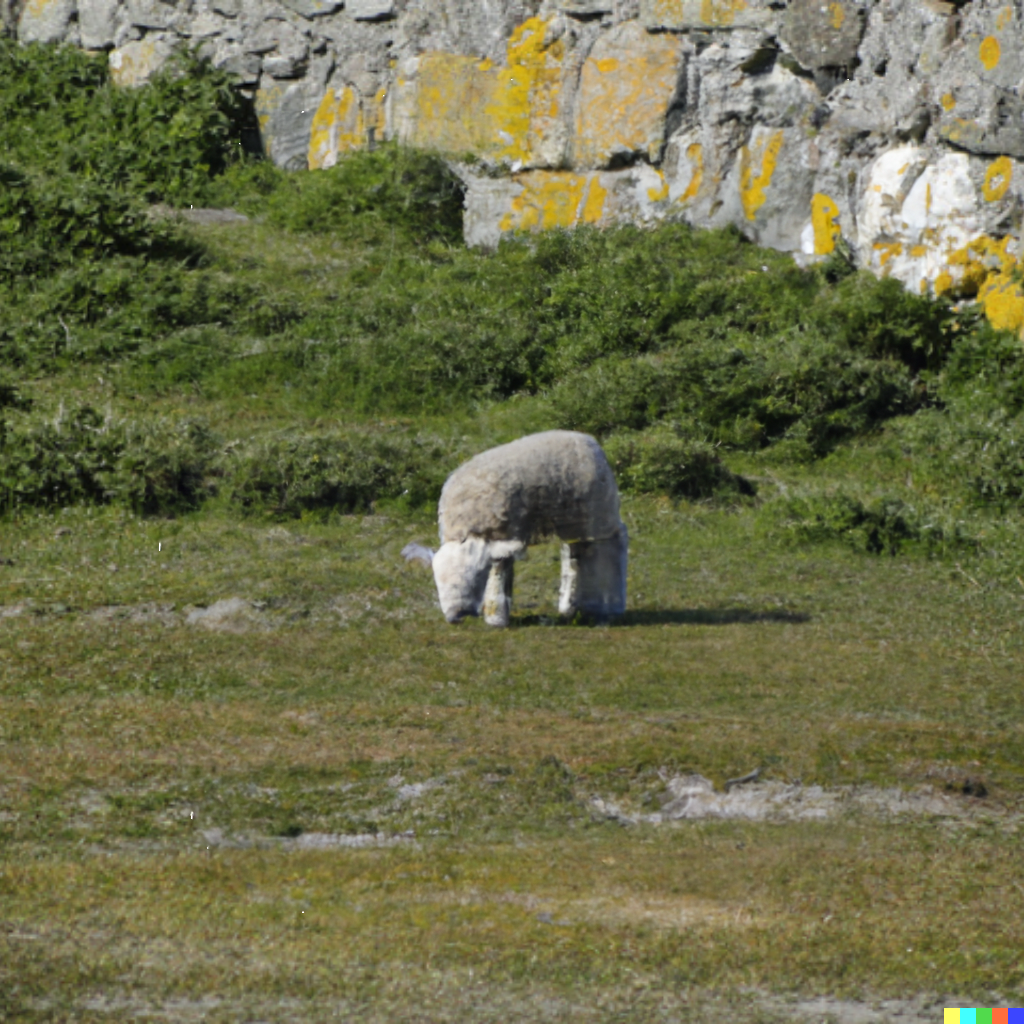
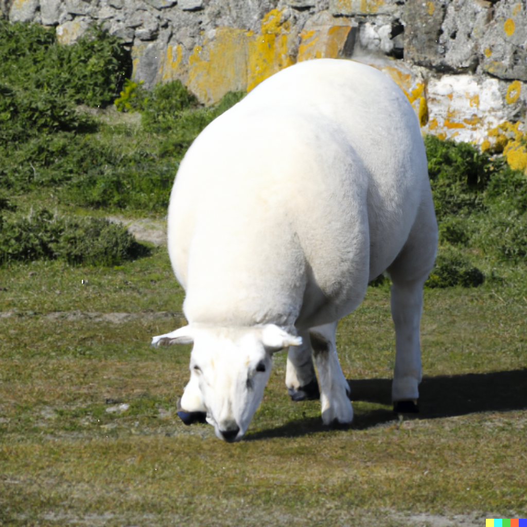
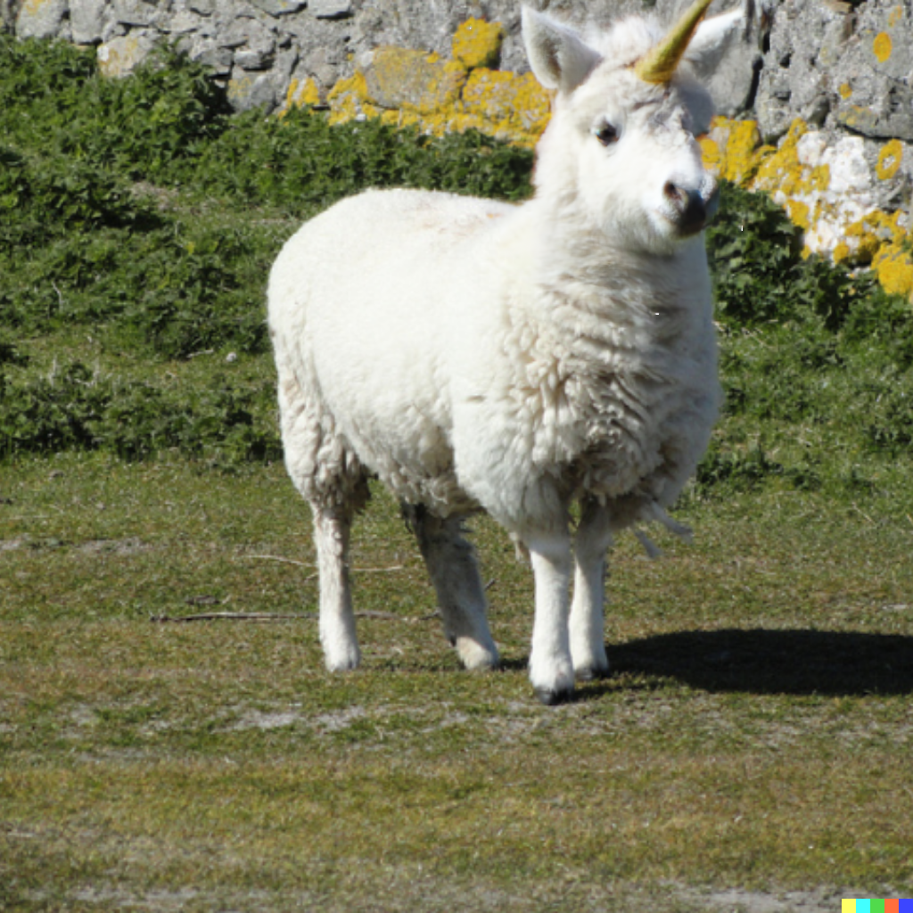
In the density function this is captured as

\[f_B(\mathbb{Y}) = \begin{cases} 1 - r & \text{if } \mathbb{Y} = \emptyset, \\ r p(y) & \text{if } \mathbb{Y} = \{ \mathbf{y} \}, \\ 0 & \text{if } |\mathbb{Y}| > 1, \end{cases}\]

where

\[p(y) = p_{\text{cls}}(y) p_{\text{bbox}}(y),\]

describes the class and bounding box distribution of the object \(y\), respectively. In this work, we have set \(p_{\text{bbox}}(y)\) to be a multinomial Gaussian over the bounding box parameters, and let the detector predict the means and covariances.

Modeling multiple objects

Naturally, in object detection, there can be multiple objects in a scene.

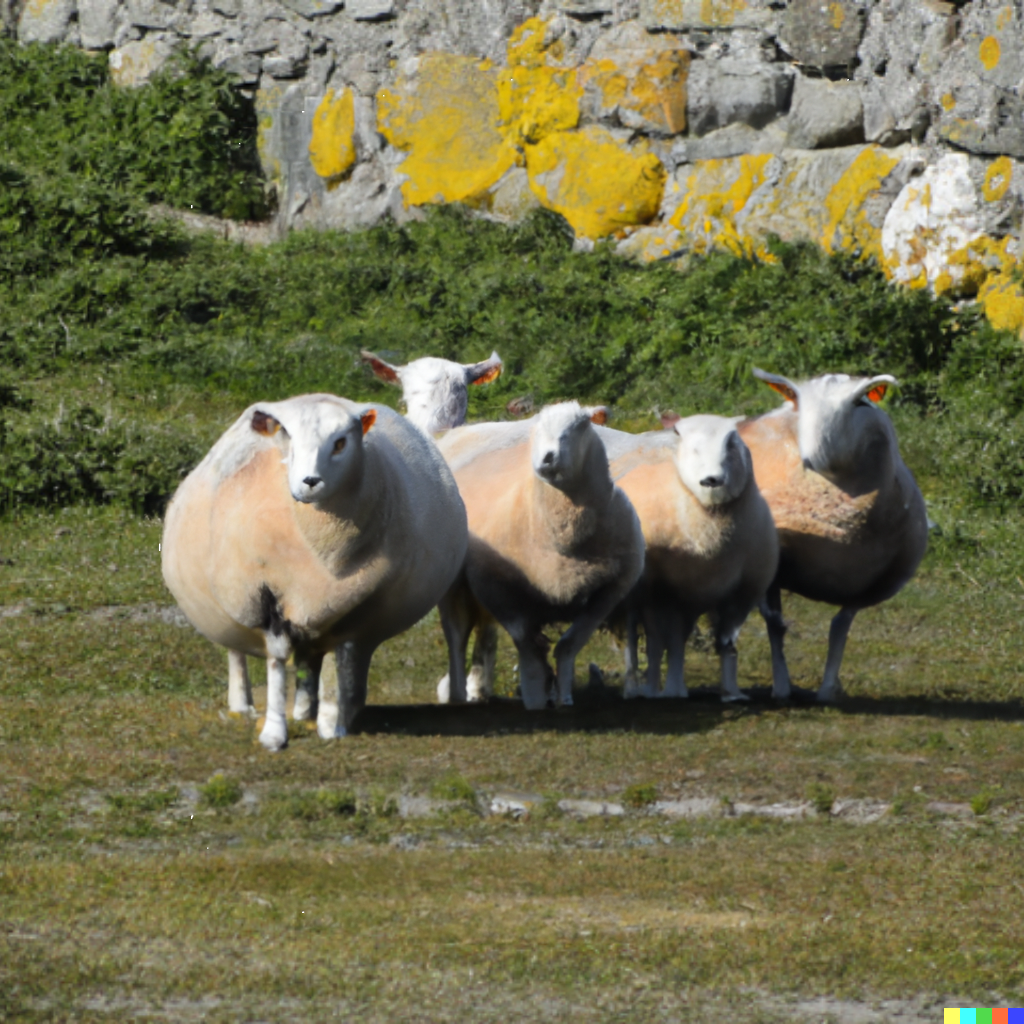
To capture all objects in a single variable, we model the objects in an image as a multi-Bernoulli RFS, which simply is the union of all Bernoulli RFSs. Its density function can be written as

\[f_{MB} (\mathbb{Y}) = \sum_{\uplus_{i=1}^{m} \mathbb{Y}_i = \mathbb{Y}} \prod_{j=1}^{m} f_{B_j}(\mathbb{Y}_j).\]

here \(\uplus_{i=1}^{m} \mathbb{Y}_i = \mathbb{Y}\) denotes all possible unions of \(m\) disjoint sets, whose union is \(\mathbb{Y}\). Effectively we sum over all possible ways of partitioning the set of objects into \(m\) sets, which is equivalent to summing over all possible ways of assigning objects to the \(m\) Bernoulli RFSs.

In practice only a few of these assignments are likely, and we can approximate the density function by summing over the \(Q\) most likely assignments. These assignments are found efficiently using Murty’s algorithm . See the paper for more details.

Modeling all objects

Another issue with using the multi-Bernoulli RFS is that it can only model up to \(m\) objects. The likelihood of any set \(|\mathbb{Y}| > m\) is zero, as any partioning will contain a set \(| \mathbb{Y_i} | > 1\), i.e., we’ll assign more than one object to a single Bernoulli RFS.

To overcome this issue, we approximate a subset of the multi-Bernoulli RFS by a Poisson Point Process (PPP) RFS with density function

\[f_{PPP}(\mathbb{Y}) = \exp (-\bar{\lambda}) \prod_{x \in \mathbb{X}} \lambda(x),\]

where \(\lambda\) is the intensity function and \(\bar{\lambda} = \int \lambda(x') dx'\).

Specifically, we take all Bernoulli RFS with existance probability \(r < \epsilon\) and model them as a PPP with intensity \(\lambda(x) = \sum_i r_i p_i(x)\). One can show that for small \(\epsilon\), say \(\epsilon = 0.1\), the density function of the PPP RFS is approximately equal to the density function of the multi-Bernoulli RFS.

We combine the PPP and MB as

\[f_{PMB}(\mathbb{Y}) = \sum_{\mathbb{Y}^U\uplus \mathbb{Y}^D = \mathbb{Y}} f_{PPP}(\mathbb{Y}^U) f_{MB}(\mathbb{Y}^D),\]

where \(\mathbb{Y}^U\uplus \mathbb{Y}^D = \mathbb{Y}\) denotes all possible ways to partition \(\mathbb{Y}\) into two disjoint sets.

We refer to the paper for effects on the optimization for finding the \(Q\) most likely assignments.

Results

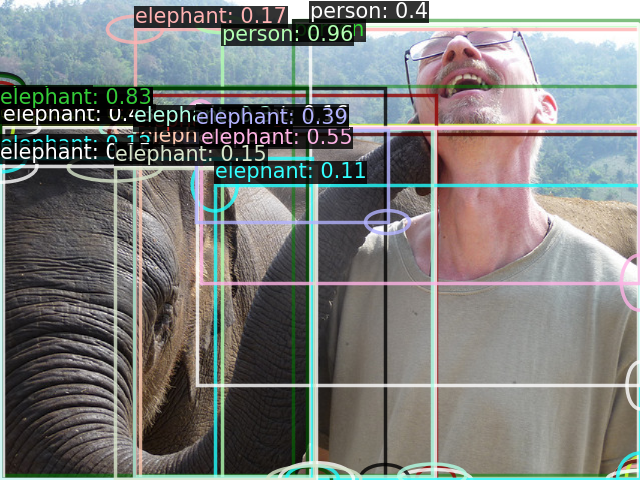
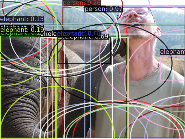
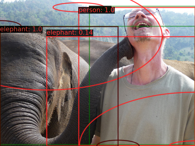
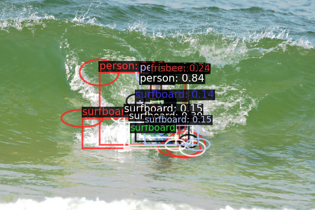
We train three detectors (DETR, RetinaNet, Faster-RCNN) using NLL and the multi-Bernoulli RFS modeling, where each detection parameterizes a Bernoulli RFS. Models are evaluated quantatively on the COCO dataset using PMB-NLL, see paper for details.